pfem

We describe here briefly the PFEM’s solution steps. It is worth to note that, excluding the FEM solution which differs for each specific application, the PFEM solution algorithm is practically independent of the physics of the problem to solve [1, 2]. A general solution scheme of the PFEM is summarized here below basing on the schematic representation of Figure 1.

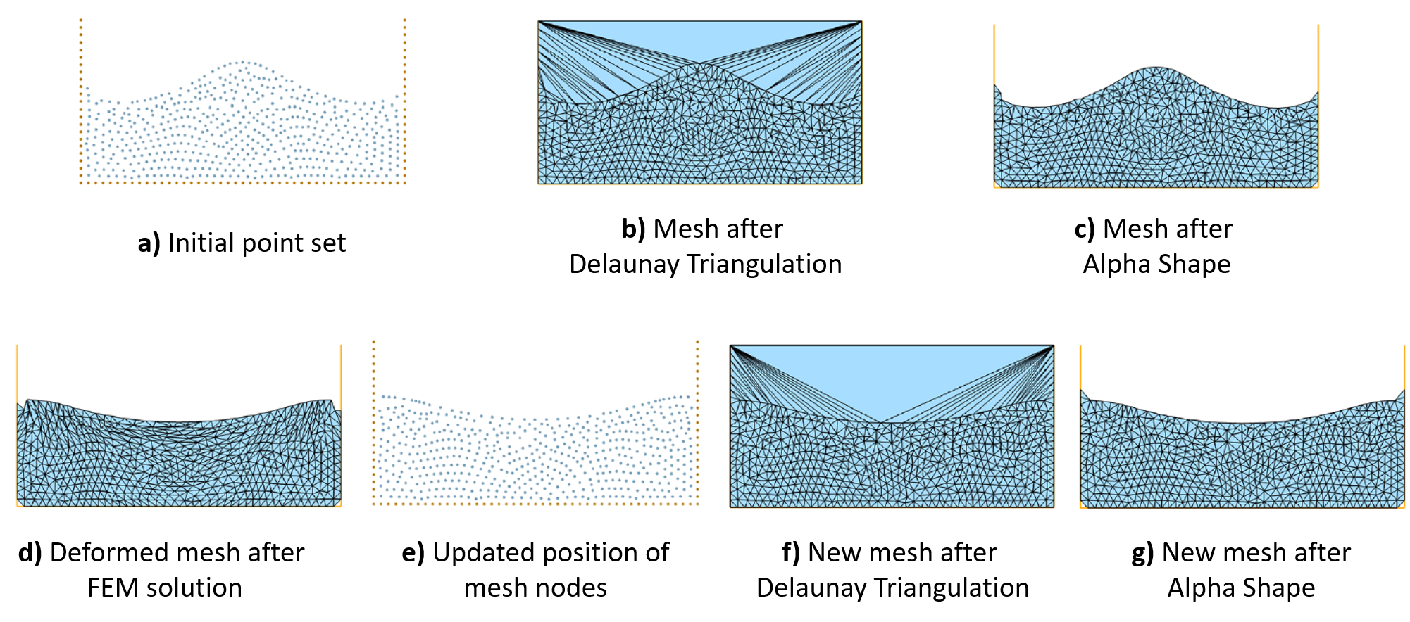Figure 1. Steps of Particle Finite Element Method [3]

The solution steps of PFEM are:

1. Fill the domain with a set of points referred to as “particles” (Fig. 1a).
2. Generate a finite element mesh using the particles as nodes (Fig. 1b).
3.  Identify the external and internal boundaries of the computational domain (Fig. 1c).
4.  Solve the Lagrangian form of the governing equations with the FEM.
5.  Update the positions of the nodes (Fig. 1d).
6.  Proceed to the next time step. If remesh is needed go to step 2, otherwise, go directly to step 5.

Figures 1e-g show the solution step for the following time instant.

In step 2, although the mesh can be regenerated with any tessellation algorithm, typically, the Delaunay triangulation is used in the PFEM. In 2D, the Delaunay triangulation has remarkable properties such as the minimization of the maximum radius of an element circumcircle and the maximization of the minimum angle among all the elements (max-min property). On the other hand, the 3D Delaunay algorithm loses some of the optimal properties of its 2D counterpart. Unfortunately, this has important consequences on the possible presence of bad quality tetrahedra in the mesh, such as zero-volume elements (slivers). The overall good properties of the Delaunay triangulation together with the availability of several fast open-source algorithms, explain the popularity of this tessellation procedure in the PFEM framework. More details about the Delaunay triangulation and its properties can be found in the PFEM review paper [3] and in the cited works.

The identification of boundaries (step 3) is necessary for the FEM solution of the governing equations. This operation is performed using the Alpha Shape method. This technique is based on the observation that the unphysical elements (those that do not belong to the real domain) are generally the largest and most distorted ones because they connect nodes that are far from each other. These are the elements that are removed from the mesh with the Alpha Shape check. More details about the use of Alpha Shape method in the PFEM are given in [3] and in the cited works.

Figure 2 provides a schematic description of the Alpha Shape method application on a two-dimensional mesh.

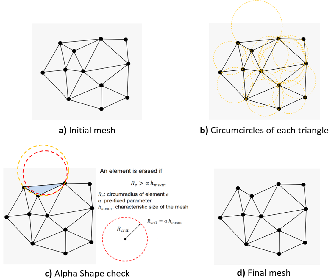
Figure 2. Application of Alpha Shape method on a two-dimensional mesh

It is also important to remark that, for those formulations using historical variables (e.g. non-linear solid mechanics), a remap of the historical variables stored at the Gauss points on the new mesh is needed before step 4.

References

[1] Idelsohn SR, Oñate E, Pin FD (2004) The particle finite element method: a powerful tool to solve incompressible flows with free-surfaces and breaking waves. Int J Numer Methods Eng 61(7):964–989
[2] Oñate E, Idelsohn SR, Pin FD, Aubry R (2004) The particle finite element method. an overview. Int J Comput Methods 1:267–307
[3] Cremonesi M, Franci A, Idelsohn SR, Oñate E (2020) A state of the art review of the Particle Finite Element Method (PFEM). Archives of Computational Methods in Engineering, 17, 1709-1735